On this page
Adversarial examples are inputs deliberately perturbed to make a model produce a wrong output, often while looking normal to a human observer. This article maps them onto the evasion category of the NIST adversarial machine learning taxonomy, walks through the attack families you need to test for (white-box, black-box, physical), explains why no single defense closes the gap, and ends with a runbook you can copy into an evaluation pipeline.
TL;DR:
- Most attacks require matching the threat model’s access level, with white-box attacks being effective only if the attacker knows the model’s architecture and weights.
- Physical and patch attacks, which simulate real-world conditions, must include transformations like printing, viewing angles, and lighting to accurately assess robustness.
- Defense strategies like adversarial training help but only against specific norms and budgets, and often reduce clean accuracy, so they need careful tuning to deployment conditions.
- Testing solely with non-adaptive, single-attack methods risks overestimating security, so including transfer, adaptive, and physical-world attacks provides a more realistic robustness assessment.
- Documenting exact inputs, model snapshots, attack parameters, and transformations is critical for reproducing failures and verifying fixes before deploying models.
Table of Contents
- What Adversarial Examples Actually Are
- Threat Models: What the Attacker Wants and What They Know
- How Attackers Generate Adversarial Examples
- Why Transferability Changes the Threat Calculation
- Why Neural Networks Are Vulnerable in the First Place
- Defenses and Their Real-World Limits
- Measuring Robustness: Metrics, Benchmarks, and a Copyable Runbook
- How Glitchive Turns Evasion Failures Into Reusable Evidence
- What to Do With This Before Your Next Model Ship
- Why Documented Failures Beat Theoretical Completeness
- Sources
- FAQ
What Adversarial Examples Actually Are
An adversarial example is the smallest input perturbation that flips a model’s prediction while staying inside a bound the attacker considers acceptable. Formally, given a model $f$, an input $x$, and a true label $y$, an attacker searches for a perturbation $\eta$ that satisfies $f(x+\eta) ew y$ (or, in the targeted case, $f(x+\eta) = y_{target}$) while keeping $|\eta|$ under some threshold $\epsilon$. That norm constraint is doing a lot of work: it’s the formal stand-in for “the change shouldn’t be obvious.”
The foundational paper on this problem demonstrated the effect with a now-famous case: a photo of a panda, given a perturbation invisible to a human eye, gets classified as a gibbon with high confidence. That example stuck in the field’s collective memory, and it’s also partly responsible for a common misconception: that adversarial examples are always tiny, imperceptible pixel noise on images. They’re not.
The norm you choose to bound $\eta$ changes what “small” even means. An $L_\infty$ constraint caps the maximum change to any single pixel or feature, which produces the classic “fuzzy noise” look. An $L_$2 constraint caps the total energy of the perturbation, which can concentrate change in a smaller region. Neither norm is a proxy for human perception; both are mathematical conveniences that sometimes correlate with it and sometimes don’t.
Beyond the pixel-noise case, several other variants matter for practitioners building test suites:
- Semantic attacks change meaningful attributes (color, pose, background) rather than adding noise, and can be just as effective at fooling a classifier.
- Spatial attacks apply rotations, translations, or warps that stay within normal-looking transformations.
- Patch attacks confine the entire perturbation to a small, visible region (a sticker, a printed square) rather than spreading it across the whole input.
- Physical attacks exist in the real world: printed patterns, altered road signs, 3D-printed objects, engineered to survive lighting and camera angle changes.
Treating adversarial examples as synonymous with invisible image noise is the single most common conceptual error in this space, and it leads teams to build test suites that miss patch and physical-world failure modes entirely.
Threat Models: What the Attacker Wants and What They Know
Testing without a threat model is like patching a lock without knowing whether you’re worried about a burglar with a crowbar or one with your house key. The NIST adversarial machine learning taxonomy, outlined on Wikipedia’s overview of the field, separates evasion attacks (adversarial examples at inference time) from poisoning attacks (corrupting training data) and model extraction or inversion attacks (stealing model behavior or leaking training data). This article focuses on evasion, but knowing where it sits in the broader map matters for scoping any security review.
Within evasion, two axes decide which attacks are realistic against your system:
- Attacker goal. An integrity attack aims for a specific misclassification (targeted) or just any wrong answer (untargeted). An availability attack tries to degrade overall performance broadly rather than hit one target. A privacy attack tries to extract training data or reverse-engineer model parameters through repeated queries, which is a different problem from evasion but often tested with the same infrastructure.
- Attacker knowledge. White-box attackers have full access to model architecture, weights, and gradients, letting them compute the exact direction that maximizes loss. Black-box attackers only get inputs and outputs (sometimes just the predicted label, sometimes confidence scores), and either query the model repeatedly to estimate gradients or train a surrogate model and attack that instead, relying on transferability to carry the attack over.
- Deployment context. A model behind a rate-limited API with no gradient exposure faces a fundamentally different risk profile than an on-device model an attacker can extract weights from directly. Testing an on-device vision model with only black-box query attacks understates its real exposure; testing a rate-limited cloud API with unrestricted white-box gradient attacks overstates it.
The practical payoff of this framing is deciding what not to test. A team shipping a cloud-hosted fraud classifier with strict rate limits doesn’t need to obsess over full white-box gradient attacks, because no real attacker gets that access. A team shipping an on-device model embedded in a mobile app should assume white-box access, because the weights ship with the app. Matching the test budget to the actual threat model, rather than running every attack against every system, is what separates a useful security review from a compliance exercise. The same framing distinction also tells you when to test for poisoning (anytime you accept external or crowdsourced training data) versus when to test for extraction (anytime your model is queryable at scale by untrusted parties) versus evasion (essentially always, once the model faces any adversarial input at inference).
How Attackers Generate Adversarial Examples
Attack algorithms split cleanly by how much they cost to run and how much model access they need. Most testing programs end up using a mix, because each family reveals different failure modes.
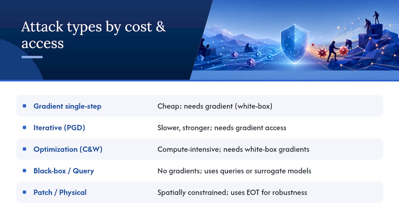
Gradient-based, single-step and iterative. The Fast Gradient Sign Method (FGSM) computes the gradient of the loss with respect to the input once and takes a single step in the direction that increases loss, scaled by $\epsilon$. It’s cheap and fast, which made it the original proof that neural networks could be fooled reliably rather than by accident. Projected Gradient Descent (PGD) iterates that same idea: take a small gradient step, project the result back inside the allowed norm ball, repeat for a fixed number of steps. PGD is slower but substantially stronger, and it’s become the de facto standard both for attacking models and, as covered below, for adversarial training. Typical setups use step counts in the range of 10 to 40 iterations, with the step size and $\epsilon$ budget tuned to the norm being tested.
Optimization-based attacks. The Carlini & Wagner (C&W) attack frames the problem as a direct optimization: minimize the perturbation size subject to a misclassification constraint, using an optimizer like Adam rather than a fixed-step gradient walk. It’s considerably more compute-intensive than FGSM or PGD, but it tends to find smaller, more effective perturbations and is often used as a stress test against defenses that look robust against cheaper attacks. If a defense holds against FGSM but collapses against C&W, that’s a strong signal the defense was tuned to the wrong attack budget rather than genuinely robust.
Black-box and query-based attacks. When gradients aren’t available, attackers turn to methods like the Square Attack, which searches for effective perturbations using randomized, structured queries rather than gradient estimation, or HopSkipJump, which estimates a decision boundary through binary search over model outputs. Both can succeed against label-only APIs with no confidence scores exposed. A parallel strategy skips querying the target entirely: train a surrogate model on similar data, attack the surrogate with white-box methods, and rely on the fact that adversarial examples transfer across model architectures and training sets far more often than intuition suggests.
Patch and physical attacks. These constrain the perturbation to a bounded region (a patch, a sticker) or require it to survive real-world capture conditions: different distances, angles, lighting, and sensor noise. That survival requirement is where Expectation Over Transformation (EOT) comes in: instead of optimizing a perturbation against one fixed image, EOT optimizes it against a distribution of transformed versions of that image, so the resulting patch keeps working after being printed, photographed, and viewed at an angle.

The practical takeaway for anyone building a test harness: an attack that only works digitally, in a single fixed view, on a model with exposed gradients tells you almost nothing about how the same model behaves against a printed sticker photographed from across a parking lot. Each attack family exercises a different assumption, and skipping one leaves a blind spot in the evaluation.
Why Transferability Changes the Threat Calculation
Transferability is the property that makes black-box attacks practical at all: an adversarial example crafted against one model frequently fools a completely different model trained on different data, provided both models learned similar decision boundaries for the task. This matters because it means an attacker never needs your production weights. They can train a rough surrogate on public data, craft attacks against it, and fire those same inputs at your deployed system with a meaningful success rate.
A handful of demonstrations from the research literature illustrate what this looks like outside a lab notebook:
- Printed and re-photographed adversarial images kept fooling classifiers after going through a camera, showing the perturbation survives the print-and-recapture pipeline, not just a raw digital file.
- Small adversarial stickers, placed on or near an object, have been shown to shift a classifier’s or detector’s output for that object without covering it.
- Perturbations physically applied to 3D-printed objects and road-sign-style surfaces kept their effect across multiple viewing angles, a direct consequence of training with EOT-style transformation robustness.
Each of these demos teaches the same lesson: an attack tested only in the clean, single-image digital case will overstate how safe the system is once it faces a camera, a lens, and ambient light. Any test harness for a vision system deployed in the physical world (autonomous driving perception, retail security cameras, drone-based inspection) needs to include physical transforms and EOT-style robustness checks, not just digital-domain perturbation budgets.
Why Neural Networks Are Vulnerable in the First Place
Two explanations dominate the current understanding, and they point toward different mitigation strategies, which is exactly why the field hasn’t converged on one fix.
The first is the linearity argument from the original FGSM paper: even though neural networks stack nonlinear activation functions, many of them behave close to linearly across the small regions relevant to a single perturbation step, especially in high-dimensional input spaces. A tiny, coordinated nudge to thousands of input features, each too small to notice individually, can add up to a large shift in the model’s output. High dimensionality is the multiplier here: the more input features a model consumes, the more room an attacker has to spread an imperceptible perturbation across all of them while still moving the decision boundary substantially.
The second explanation, from the non-robust features line of work, argues that models learn to rely on genuinely predictive but visually meaningless patterns in the training data, patterns that correlate with the label in the training distribution but don’t correspond to anything a human would call the “real” signal. A model trained on that data isn’t malfunctioning when it follows those patterns; it’s doing exactly what standard training rewards it to do. Adversarial perturbations exploit those brittle correlations directly.
For practitioners, the useful signal is behavioral: if perturbing features that seem visually irrelevant to a human causes large, confident swings in the model’s output, that’s a sign the model has learned to lean on brittle, non-robust features rather than the intended semantic signal, and standard training incentives will keep reproducing that pattern until the training objective itself changes.
Defenses and Their Real-World Limits
No defense closes this gap completely, and treating any single technique as a permanent fix is the fastest way to get blindsided later. A recent survey of the field is blunt about this: there is no silver-bullet defense, and the field functions as an ongoing arms race between attack and defense research rather than a solved problem.
Adversarial training is the most empirically durable approach available. The technique trains the model directly on PGD-generated adversarial examples alongside clean data, so the model learns to classify correctly even under perturbation. It works, but it comes with real costs: training time multiplies because generating PGD examples at every step is expensive, and models trained this way often show a measurable drop in clean accuracy compared to standard training. There’s also a matching problem: adversarial training tuned to one norm and epsilon budget provides little protection against attacks using a different norm or a larger budget than what the model trained against, so the training budget has to reflect the deployment threat model, not an arbitrary convenient number.
Input transforms and preprocessing (JPEG compression, randomized resizing, feature squeezing) can knock out weak attacks by disrupting the precise pixel-level structure an optimizer relied on. They tend to fail against adaptive attackers who know the transform is in place and simply optimize through it, and several published transform-based defenses have been broken this way once attackers accounted for the preprocessing step in their optimization loop.
Certified defenses offer a genuinely different guarantee: instead of empirical robustness against known attacks, they provide a provable bound. Randomized smoothing, for example, can certify that no perturbation within a given radius changes the prediction, which is a mathematically real guarantee rather than an observed pattern. The catch is scalability: certified radii tend to be smaller than the perturbation budgets attackers realistically use, and the certification overhead grows with model and input size, which has kept certified defenses out of many large-scale production systems.
Detection and ensemble approaches try to flag adversarial inputs before they reach the model, or combine multiple models to make attacks harder to transfer across the whole ensemble. Both run into the same wall: an adaptive attacker who knows the detection mechanism or ensemble composition can often optimize directly against it, and defenses evaluated only against non-adaptive attacks routinely look far stronger than they actually are. This is the mechanism behind gradient masking: a defense that appears to work only because it obscures or flattens the gradient signal an attacker would need, without actually making the underlying decision boundary more robust. Testing exclusively with gradient-based attacks against such a defense produces a false sense of security, because the masked gradient blocks the attack method without addressing the vulnerability.
The operational rule that falls out of all this: never validate a defense using only the attack it was designed to stop. Run transfer attacks from independently trained surrogate models, run adaptive white-box attacks that assume full knowledge of the defense, and treat any defense that only survives non-adaptive testing as unproven.
Measuring Robustness: Metrics, Benchmarks, and a Copyable Runbook
Robustness isn’t a single number, and treating it as one is how teams end up shipping a model that “passed” evaluation and failed in production anyway. Four metrics matter for most evaluation programs:
- Robust accuracy under a fixed norm budget — accuracy measured specifically against attacks constrained to $\epsilon$, the number that should always be reported alongside the accuracy figure itself, since robust accuracy at $\epsilon=0.01$ and $\epsilon=0.1$ describe entirely different security postures.
- Certified bound — the provable radius within which no perturbation can change the prediction, where applicable.
- Worst-case failure rate — the failure rate against the strongest attack you tested, not the average across a mix of weak and strong attacks, since averaging hides exactly the failure mode you’re trying to catch.
- Query efficiency of the attacks used — how many queries a black-box attack needed to succeed, which tells you how exposed a rate-limited production API actually is.
Here’s a runbook that turns those metrics into a repeatable process:
- Define the threat model first. Write down attacker goal, knowledge level, and deployment context before selecting a single attack algorithm.
- Select attacks and budgets that match that threat model. Pair white-box gradient attacks with the epsilon and norm you expect in deployment; add black-box query attacks if the model is externally reachable; add physical/EOT tests if the model processes real-world captured input.
- Run adaptive attacks against every defense in place, assuming the attacker knows the defense mechanism, not just naive attacks against an undefended model.
- Record full artifacts for every run: exact model weights and checkpoint, preprocessing pipeline, RNG seeds, attack hyperparameters, and any input transformations applied, so a failure can be reproduced and triaged later rather than debugged from memory.
- Compare results against the worst-case metric, not the average, and flag any regression against the previous evaluation run as a candidate for rollback.
Pro Tip: Log the exact random seed used for every attack run. Adversarial optimization is sensitive to initialization, and without the seed you can spend hours failing to reproduce a failure your own pipeline generated last week.
| Test category | What it catches | Minimum artifact to log |
|---|---|---|
| White-box worst-case (PGD, C&W) | Full-knowledge attacker exploiting exposed gradients | Model checkpoint, epsilon, norm, step count |
| Transfer / black-box (surrogate, Square Attack) | Realistic external attacker without gradient access | Surrogate architecture, query budget, success rate |
| Physical / EOT | Real-world capture conditions (print, angle, light) | Transform distribution used, physical medium tested |
For teams that need to go deeper into building and hosting the test tooling itself, guidance on preparing reproducible developer artifacts covers the same reproducibility discipline this runbook depends on, applied to a broader engineering context.
How Glitchive Turns Evasion Failures Into Reusable Evidence
Glitchive exists to document AI failures with enough detail that a team facing a similar problem can act on it instead of starting from theory. For an evasion failure specifically, that means capturing the case with the same rigor an adversarial robustness test demands: the exact input, the model snapshot at the time of failure, the attack or transformation that triggered it, and the fix that was verified to close the gap.
An illustrative structure for documenting an adversarial evasion incident, in the format Glitchive uses across its case library, looks like this:
- Summary: what input caused what misprediction, and under what deployment conditions.
- Root cause factors: which threat category applies (white-box, black-box, physical) and which underlying vulnerability was exploited.
- Remediation applied: the specific defense or process change implemented, and its measured trade-offs.
- Verification results: what re-testing confirmed the fix actually held, including whether adaptive attacks were used to check for gradient masking.
| Field to capture | Why it matters |
|---|---|
| Exact input and model snapshot | Enables reproduction of the exact failure |
| Attack method and parameters (epsilon, norm, steps) | Distinguishes threat-model-relevant failures from edge cases |
| Environmental transforms tested | Confirms whether the fix holds under physical conditions |
| Verification method used to confirm the fix | Prevents shipping a fix that only masks the symptom |
That structure is a template, not a specific claim about any documented case. Teams building their own internal incident log for adversarial failures can adapt those same four fields directly.
What to Do With This Before Your Next Model Ship
Three habits separate teams that catch adversarial failures early from teams that find out in production. First: never validate a defense using only the attack it was built to stop; always add transfer and adaptive attacks. Second: match your test budget (epsilon, norm, physical transforms) to your actual deployment threat model, not a convenient default. Third: log full reproduction artifacts (weights, seeds, attack parameters) for every evaluation run.
Escalate immediately if a model’s confidence stays high on inputs that fail robust-accuracy checks, or if a defense that passed non-adaptive testing hasn’t yet faced an adaptive attacker. Treat adversarial evaluation as continuous, not a one-time gate before launch, and document every failure with enough detail that the next model version can be checked against it.
Why Documented Failures Beat Theoretical Completeness
Reading a survey of attack algorithms tells you what’s possible. Reading a documented case of a specific model failing against a specific perturbation, with the exact fix that closed the gap, tells you what to actually check before your own model ships. That difference is why case evidence matters more for prioritization than another taxonomy paper: it turns an abstract vulnerability into a concrete test you can run this week.
Glitchive’s methodology is built around that gap. Practitioners who’ve hit an adversarial failure worth documenting, or who’ve found a fix worth verifying, are the reason the case library stays useful rather than theoretical. If you’ve seen a production model fail this way, the corrections process exists to keep every published case accurate as new evidence comes in.
— GH
Sources
- Explaining and Harnessing Adversarial Examples
- Attacking machine learning with adversarial examples — OpenAI
- A Survey of Adversarial Examples in Computer Vision: Attack, Defense, and Beyond
FAQ
What is an adversarial example?
An adversarial example is an input deliberately modified, usually with a small, bounded perturbation, to cause a machine learning model to produce an incorrect prediction, often while looking unremarkable to a human observer.
What is adversarial behavior in machine learning?
Adversarial behavior refers to any intentional attempt to manipulate a model’s input, training data, or query pattern to force an incorrect output, steal model information, or degrade performance, spanning evasion, poisoning, and extraction attacks.
Can you give an example of an adversarial attack?
A classic example is a printed sticker placed on a stop sign that causes an image classifier to label it as a speed limit sign, or a photo perturbed just enough to make a model report a completely different object with high confidence, as demonstrated with FGSM’s original panda-to-gibbon result.
What does “adversarial” mean in an AI security context?
In AI security, “adversarial” describes any input, data point, or interaction deliberately engineered by an attacker to exploit a model’s weaknesses, as opposed to naturally occurring noise or errors the model might encounter by chance.
Is there a single defense that stops adversarial examples?
No. Surveys of the field consistently find no silver-bullet defense; adversarial training, certified defenses, and input transforms each help against specific threat models but carry trade-offs and can be bypassed by adaptive attackers.