On this page

Dataset shift means the joint distribution your model was trained on no longer matches the distribution it faces in production, formally P_train(X, y) ≠ P_test(X, y). That single inequality breaks the i.i.d. assumption underlying almost every standard training procedure, and it does so silently: no exception gets thrown, no pipeline fails, the model just gets quietly worse at its job.
Whether this demands active remediation depends on effect size and your business’s tolerance for degraded predictions. A small calibration drift on a low-stakes recommendation model is background noise. The same drift on a fraud model or a clinical triage tool is an incident. Moreno-Torres et al. gave the field its canonical taxonomy for classifying these shifts, ADWIN remains the standard adaptive-window detector for catching them in streaming data, and Glitchive exists specifically to document the moment teams got this wrong in production.
If your dashboards flag anomalous performance right now, run these checks in the first 30 to 60 minutes:
- Confirm upstream schema and telemetry are intact before touching the model.
- Compare current feature distributions to a recent training-window baseline.
- Check whether errors cluster in specific segments or spread uniformly.
- Verify label pipeline latency hasn’t silently changed evaluation windows.
- Hold off on retraining until you’ve ruled out a data-quality bug.
That last point matters most. A broken ETL job, a renamed field, or a logging outage can mimic dataset shift almost perfectly. True shift is a change in the world; a data-quality error is a change in your instrumentation. Confuse the two and you’ll either retrain on garbage or ignore a real problem while blaming your pipeline.
Key Takeaways
Dataset shift degrades model performance silently, and separating genuine distributional change from an engineering bug is the single highest-leverage diagnostic skill a production ML team can build.
| Point | Details |
|---|---|
| Formal definition | Dataset shift means P_train(X, y) ≠ P_test(X, y), breaking the i.i.d. assumption behind standard training. |
| Classify before you fix | Covariate shift, label shift, and concept drift each need a different mitigation, so diagnose the type first. |
| Rule out engineering first | Run a schema and telemetry health check before touching the model; many “shifts” are pipeline bugs. |
| Use the right test for the job | KS suits single-feature checks, MMD and Wasserstein distance handle multivariate or outlier-heavy data. |
| Gate retrains with humans | Add a human-in-the-loop validation gate and staged rollout before any automated retrain reaches full traffic. |
Table of Contents
- What Are the Main Types of Dataset Shift?
- What Causes Dataset Shift in Production Systems?
- How Do You Detect Dataset Shift in Production?
- What Are the Best Ways to Mitigate Dataset Shift?
- A Worked Example and Deployment Checklist
- What Are the Limits of Dataset Shift Detection?
- What I’ve Learned Watching Shift Break Production Systems
- Primary Sources for Dataset Shift and Concept Drift
- Sources
- FAQ
What Are the Main Types of Dataset Shift?
Practitioners lump too much under “shift.” The canonical framing from Moreno-Torres et al. splits it into distinct types, each breaking a different assumption and calling for a different fix.
- Covariate shift. P(X) changes but P(y|X) stays fixed. Your input distribution moves, but the underlying relationship between features and labels doesn’t. Mitigation hint: importance weighting or reweighting training samples to resemble the new input distribution.
- Prior probability (label) shift. P(y) changes while P(X|y) holds constant. The base rate of your classes shifts, for instance fraud becoming rarer or more common, without the feature signature of fraud itself changing. Mitigation hint: recalibrate decision thresholds or apply label re-weighting rather than retraining features from scratch.
- Concept drift. P(y|X) itself changes over time. The same input now maps to a different correct output. This is the hardest case because your features can look identical while the ground truth relationship has moved. Mitigation hint: online learning, sliding-window retraining, or ensemble methods that track recent data more heavily.
- Sample selection bias / domain shift. The training data was never a fair sample of the deployment population to begin with, often due to how it was collected or filtered. Mitigation hint: bias correction via inverse propensity weighting, or collecting a genuinely representative validation set.
- Concept evolution. New classes or categories appear that didn’t exist in training, common in fraud and malware detection where adversaries invent new attack types. Mitigation hint: open-set recognition or periodic retraining with expanded label taxonomies.
- Delayed labels. Not a distribution change per se, but a measurement problem: your ground truth arrives too late to detect concept drift in real time. Mitigation hint: use proxy labels or shorter-horizon surrogate metrics while waiting for true labels.
These categories overlap more than textbooks suggest. Sample selection bias frequently masquerades as covariate shift because both manifest as a changed P(X), and you often can’t tell them apart without knowing how your training data was originally collected.
What Causes Dataset Shift in Production Systems?
Shift rarely comes from one dramatic event. It’s usually a slow accumulation of small mismatches between the world your model learned and the world it now operates in.
Common mechanisms include non-stationarity (the underlying process genuinely changes over time), selection bias baked in at collection time, measurement or instrumentation changes (a sensor gets recalibrated, an SDK version changes how events are logged), user-behavior shifts, seasonal effects, adversarial adaptation, and outright changes in label distribution. Each leaves a different fingerprint.
A few illustrative examples follow, each a composite pattern rather than a documented incident:
- Illustrative example, image classification: A model trained on daytime photos degrades when a product update shifts users toward nighttime uploads. Feature distribution moves (covariate shift), but the visual concept of “cat” versus “dog” hasn’t changed.
- Illustrative example, malware detection: Attackers deliberately restructure payloads to evade a classifier trained on last year’s samples. This is concept evolution combined with adversarial concept drift, and it’s why security models decay faster than almost any other model class, a pattern well documented in the concept drift literature.
- Illustrative example, customer churn: A pricing change shifts which customers churn and why, altering P(y|X) even though the feature set (tenure, usage, support tickets) stays identical.
- Illustrative example, labeling delay: A credit risk model’s true labels (default or no default) take 90 days to materialize, meaning drift can go undetected for a full quarter before anyone notices the gap between predicted and realized outcomes.
The business impact runs through three channels: false positives that erode user trust, missed true positives that cost revenue directly, and, in regulated domains, compliance exposure when a degraded model keeps making decisions nobody is actively supervising.
How Do You Detect Dataset Shift in Production?
Detection means watching the right signals, running the right statistical tests, and having a clear order of operations before you touch the model.
Monitor these signal categories continuously: model performance metrics (error rate, calibration curves), feature-distribution metrics per input, input schema validity, upstream event rate anomalies, data freshness, and label latency. A spike in any one of these, in isolation, usually means an engineering problem. A correlated move across several is a stronger shift signal.
For quantifying distributional change, four tests dominate practice. The Kolmogorov-Smirnov (KS) test compares empirical cumulative distributions for a single feature and works well for continuous univariate data, though it loses power in high dimensions. Maximum Mean Discrepancy (MMD) compares distributions in a kernel-embedded space and handles multivariate and non-Gaussian data better than KS, at higher computational cost. Wasserstein distance measures the “cost” of transforming one distribution into another and is more robust to outliers than KL divergence. KL divergence is fast to compute but requires density estimates and can blow up when distributions have non-overlapping support. The KDD ‘26 benchmarking framework documents the trade-offs among these approaches in detail.
For streaming detection, ADWIN (adaptive windowing) adjusts its comparison window size automatically as it detects change, making it a standard choice for continuous production pipelines. KSWIN applies the KS test within an adaptive window for lighter-weight streaming checks. CUSUM and DDM track cumulative deviation and error-rate changes respectively, both useful when you need a lightweight alarm rather than a full distributional comparison.
Follow this order when an alert fires:
- Run an engineering health check: schema validity, null rates, upstream service status.
- Run univariate KS or MMD tests on the specific features flagged.
- Check model performance metrics against a rolling baseline.
- Where possible, sample and label a small batch to check for conditional shift in P(y|X), not just P(X).
- Inspect label quality itself, since noisy or delayed labels can look identical to concept drift.
Pro Tip: Set your drift thresholds using a rolling historical baseline, not a single fixed number. A threshold tuned on last year’s traffic patterns will fire constantly during any seasonal cycle you didn’t account for.
Escalate to retraining only after steps 1 through 3 rule out an engineering cause and the effect size crosses your business-defined tolerance. Escalate to manual investigation when the signal is ambiguous or confined to a small segment.
What Are the Best Ways to Mitigate Dataset Shift?
Mitigation choices split naturally by where they intervene: before training, at inference time, or as an ongoing adaptation loop. Picking the wrong one for your shift type wastes engineering effort and sometimes makes things worse.
Training-time methods assume you can retrain or reweight before deployment. Importance weighting reweights training examples so they resemble the target distribution, and it works only under the covariate shift assumption that P(y|X) stays invariant. Domain adaptation techniques learn representations less sensitive to the shifted input space, useful when you have some unlabeled target-domain data but no labels. Robust loss functions (Huber loss, focal loss) reduce sensitivity to distributional outliers at some cost to peak accuracy on clean data. Data augmentation simulates plausible future shifts during training, cheap to apply but only as good as your ability to anticipate what will actually change.
Inference-time methods act without retraining. Test-time adaptation adjusts model behavior using statistics from the incoming batch, useful for sudden but temporary shifts. Confidence calibration recalibrates output probabilities so a model’s uncertainty estimates stay honest even as inputs drift, cheap to apply but doesn’t fix underlying accuracy loss. Rejection or abstention thresholds let a model decline to predict on inputs it’s unsure about, trading coverage for reliability, essential in any high-stakes deployment where a wrong answer is worse than no answer.

Ongoing adaptation methods treat drift as continuous rather than a one-time event. Online learning updates model weights incrementally as new labeled data arrives, appropriate when concept drift is frequent and labels arrive quickly. Sliding-window retraining periodically refits on only the most recent data, discarding stale patterns, simple to implement but wasteful of historical signal if drift is actually mild. Ensembles that weight recent models more heavily adapt smoothly without discarding older knowledge outright. Continual learning frameworks aim to retain old knowledge while incorporating new patterns, though they remain harder to operate reliably than the simpler alternatives.
The assumptions matter more than the method names. Importance weighting is worthless if P(y|X) has actually changed, since it only corrects for a shifted P(X). Online learning is dangerous if your labels are noisy, since it will happily learn the noise as fast as it learns the signal.
Validating under shift requires different tooling than standard cross-validation. Importance-weighted cross-validation corrects for the fact that your validation set no longer represents the deployment distribution. Covariate-robust metrics evaluate performance conditioned on distributional buckets rather than in aggregate. Leave-one-dataset-out validation, the protocol the KDD ‘26 evaluation framework proposes for detector tuning, holds out an entire data source during validation to test whether a detector generalizes beyond the specific environment it was tuned on rather than memorizing quirks of one benchmark.
Retraining frequency should follow business tolerance rather than a fixed calendar. A fixed monthly retrain wastes compute on stable periods and reacts too slowly during volatile ones. A detector-triggered retrain, fired when a drift metric crosses a pre-agreed threshold, matches effort to actual need but requires the detection layer described above to be trustworthy first.
Dataset shift detection differs from out-of-distribution (OOD) detection and general anomaly detection in scope and intent. OOD detection flags individual inputs that fall outside the training manifold, useful for rejecting a single bizarre request. Anomaly detection flags rare events within a presumed-stable distribution. Dataset shift detection asks a population-level question: has the overall distribution moved, even if any single input looks perfectly normal? You need all three in a mature system, but they answer different questions and fire on different timescales.
A Worked Example and Deployment Checklist
Here’s a compact illustrative example, not a documented incident, showing how the pieces fit together in pseudo-code:
baseline = load_reference_distribution(feature="avg_session_length")
current = get_production_window(hours=24)

ks_stat, p_value = kolmogorov_smirnov_test(baseline, current)
mmd_score = compute_mmd(baseline, current, kernel="rbf")

if p_value < 0.01 and mmd_score > threshold:
    flag_candidate_shift()
    run_engineering_healthcheck()  # rule out ETL/schema issues first
    if healthcheck_passes():
        apply_importance_weighting(current_batch)
        schedule_verification_retrain()
This flags the feature, checks for an engineering cause first, and only then applies a correction, exactly the order the diagnosis runbook above recommends.
A 10-item deployment checklist you can paste into a runbook:
- Confirm schema and telemetry integrity before anything else.
- Pull a 24 to 72 hour production feature sample.
- Run KS or MMD against a recent training-window baseline.
- Check model error rate and calibration against a rolling baseline.
- Segment errors to check whether shift is localized or global.
- Sample and label a small batch to probe P(y|X), not just P(X).
- Inspect label pipeline latency and label quality.
- Decide: engineering fix, threshold recalibration, or retrain.
- If retraining, validate on a leave-one-dataset-out holdout before deployment.
- Set a rollback trigger tied to a specific post-deployment metric threshold.
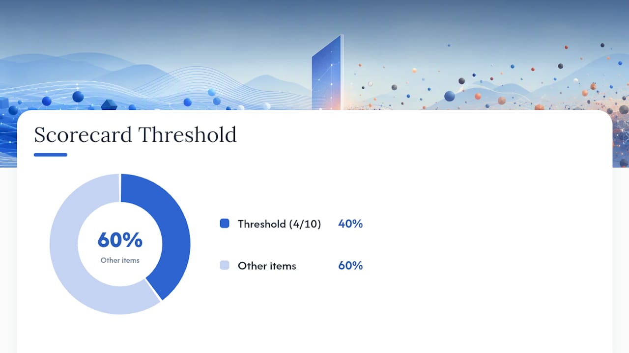
A 10-item scorecard to distinguish true shift from a data-quality incident: score each item yes or no. Did the alert correlate with a deployment or config change? Is the affected feature single or multiple? Did schema validation pass? Are null rates stable? Did upstream event volume stay constant? Does the shift persist across multiple time windows? Do labels (where available) confirm a real outcome change? Is the pattern consistent across independent data sources? Would the same drift show up in a shadow pipeline? Has a human reviewer manually confirmed the pattern? Four or more “no” answers point toward a data-quality bug, not genuine shift.
When you do confirm a real shift event, document it the way Glitchive’s case studies do: capture the timeline, the root cause, the specific mitigation applied, the measured outcome, and a permanent citable link so the next engineer who hits the same pattern doesn’t start from zero.
What Are the Limits of Dataset Shift Detection?
No detector catches everything. Shifts without any labeled feedback are fundamentally hard to confirm, since you’re often inferring P(y|X) change from proxies rather than ground truth. Label delay compounds this: by the time true labels arrive, the shift may have already evolved past what you detected.
Practitioners also lean too hard on synthetic benchmarks. The KDD ‘26 framework found that detectors tuned on synthetic drift patterns routinely overstate real-world performance, since synthetic data omits the noise and irregular nonstationarity that real production streams contain. Common mistakes include retraining on noisy labels without auditing them first, ignoring an upstream schema change while chasing a phantom model problem, tuning a detector’s thresholds on the same dataset used to evaluate it, and conflating anomaly detection with shift detection when they answer different questions.
Pro Tip: Put a human-in-the-loop validation gate before any automated retrain reaches production, and roll it out to a small traffic slice first. A noisy retrain triggered by a false alarm can do more damage than the drift it was meant to fix.
What I’ve Learned Watching Shift Break Production Systems
Teams treat dataset shift as a modeling problem when it’s usually a monitoring problem in disguise. The models are rarely the weak link; the absence of a fast, cheap way to compare today’s inputs against yesterday’s is.
If you invest in one thing, invest in unlabeled-data distribution monitoring paired with a small, fast labeled verification pipeline. The monitoring catches the signal early; the verification pipeline stops you from retraining on a false alarm.
Primary Sources for Dataset Shift and Concept Drift
- Dataset Shift in Machine Learning (MIT Press) provides the unifying theoretical framework connecting shift to transfer and active learning.
- Moreno-Torres et al. (2012) established the canonical taxonomy used throughout this article.
- The KDD ‘26 evaluation framework standardizes detector benchmarking and warns against synthetic-only validation.
Sources
- Dataset Shift in Machine Learning
- A unifying view on dataset shift in classification (Moreno-Torres et al., 2012)
FAQ
What Is a Dataset?
A dataset is a structured collection of examples, typically feature values paired with an optional label, used to train, validate, or test a machine learning model.
What Is Covariate Shift?
Covariate shift is a type of dataset shift where the input distribution P(X) changes between training and production while the underlying relationship P(y|X) stays the same.
What Are the Four Main Types of Data Sets?
In machine learning workflows, data is typically split into training, validation, test, and production (live) datasets, each serving a distinct role in building and monitoring a model.
What Is the Difference Between a Dataset and a Database?
A dataset is a specific collection of data used for a task like model training, while a database is a broader, often queryable system designed to store, organize, and retrieve data across many uses.
How Is Dataset Shift Different From Out-of-Distribution Detection?
Dataset shift detection asks whether the overall population distribution has moved, while out-of-distribution detection flags individual inputs that fall outside the training data’s manifold.